Discontinuous piecewise linear interpolation in MIPs

I received some questions and feedback from the post here: http://yetanothermathprogrammingconsultant.blogspot.com/2015/10/piecewise-linear-functions-in-mip-models.html. Here are some “back to basics” notes  on modeling piecewise linear functions. I only look at the easy case: one dimensional only, i.e. y=f(x). This is all simple stuff but it may be useful to show all the different cases in a row. (At least I can now simplify answering a lot of emails by referring to this post).

Continuous, bounded convex case

An example is:

The slope and the intercept can be calculated as:

If the model is convex i.e. if we somehow maximize y using the above curve, then we simple can write:

If we are minimizing y then the curve needs to be sloping up. E.g. in electricity power generation models we often see quadratic cost (to be minimized) as function of output. Of course the sign in the BoundY(s) equation need to be flipped to ≥ in such a case. (Here we have also a possible opportunity to formulate the problem as a MIQP – often we see that a piecewise linear model performs better.)

If we can exploit this “convexity”, then we don’t need any additional discrete variables.

The fact that we want to bound x between 10 and 45 is easily handled by adding lower and upper bounds to x. This case also deals directly with the unbounded case (see below for a further discussion of this), by just not adding a bound on x.

Continuous, bounded non-convex case

Now assume we don’t have convexity (for instance, we are not maximizing y using the above curve; e.g. because y represents cost). This means we need discrete variables.

Using binary variables σ_s and additional continuous variables xs_s one could write:

Here xs_s= 0 if x is outside of the selected segment s, and xs_s= x if x is inside this segment s. The selection of a segment is indicated by σ_s=1. In the math above, variables are red and data (constants) are displayed in blue. We see quickly we do not multiply variables by variables and thus this is nicely linear.

This is a little improvement over the discussion in http://yetanothermathprogrammingconsultant.blogspot.com/2015/10/piecewise-linear-functions-in-mip-models.html as we simplified the equation CalcY by doing some data manipulation in advance. In general that is a good idea: it moves complexity away from the equations which are the most difficult to debug. I am a big proponent of keeping the equations as simple as possible.

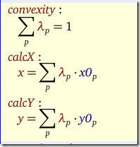
With SOS2 variables λ_p we can do the following. The data requirements are slightly different. We need a table like:

This will allow us to formulate:

Note that we have called here the equation that sums up the λ’s to one: “convexity”. This is the typical name for this equation (even though we are dealing with a non-convex case).

In the following sections we will assume that σ_s∈ {0,1} are binary variables and λ_p are SOS2 variables.

Semi-Continuous, bounded non-convex case

Now assume the data looks like:

This is not so unusual. You get a discount on the (total) price when ordered more than some limit.

The binary variable formulation does not change at all: we can model this directly using the three segments in the table.

The SOS2 variable formulation needs some extra points. Our input for the SOS2 version becomes:

Notice that in this formulation it may be beneficial to order more than you need, just to get the discount. In some models that means modeling some salvage value (can be positive or negative) or even storing it for a future period (adding to inventory).

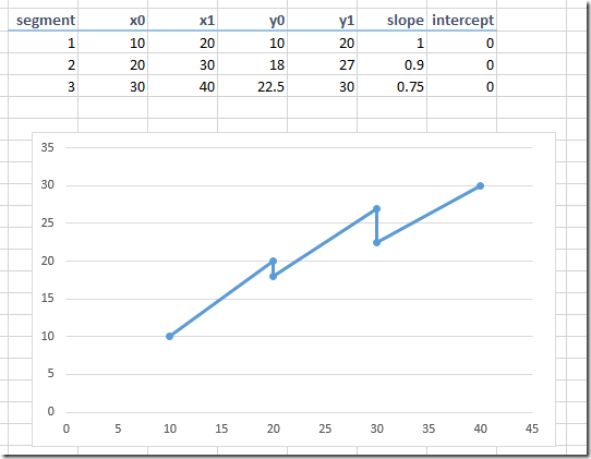
Strange case: discontinuous.

This looks crazy but actually can happen. For instance some type of power generators cannot operate at certain intervals (prohibited zones). A reason could be that amplified vibrations occur at certain operating levels.

The binary variable formulation can deal with this case directly. Unfortunately the SOS2 formulation is not applicable here.

Unbounded case

Now suppose that we don’t have an end point in the last segment (i.e. it just go on forever). Alternatively, we could not have a starting point at the beginning of the first segment.

In case of the binary variable formulation we just need to drop some inequalities dealing with the determining in which segment x is currently located.

Here NoStartPoint and NoEndPoint are appropriate subsets of s. (These sets should be empty or contain one particular element). This trick can not be used with the SOS2 formulation, but in practice that is not a problem. Usually we have some sense of a reasonable lower and upper bound on x.