In [1] a variant of the Sudoku puzzle is presented:
![]()
When we want to model this problem, we basically have three sets of constraints:
As usual we will use a binary variable [2]: \[x_{i,j,k} = \begin{cases} 1 & \text{if cell $(i,j)$ has value $k$}\\ 0 & \text{otherwise}\end{cases}\]
Using this definition, the row and column uniqueness constraints are easy using assignment constraints: \[\begin{align} & \sum_i x_{i,j,k} = 1 & \forall j,k \\ & \sum_j x_{i,j,k} = 1 & \forall i,k \\ &\sum_k x_{i,j,k} = 1 &\forall i,j\end{align}\] These assignment constraint effectively implement what is known as all-different constraints in constraint programming. See [3] for different MIP formulations for these all-different constraints.
Let's indicate a region by \(r\). We can calculate the value of a region by: \[v_r = \sum_{(i,j)|R_{i,j,r}} \sum_k k\> x_{i,j,k} \] We sum over cells in region \(r\). Now we have to add an all-different constraint: \[\text{all-different}(v_k)\] This is a slightly different all-different constraint from the ones we discussed before. Here we don't enumerate all possible values.
One way to model this, is the following. Interpret the problem as: \[ v_r \le v_{r'} - 1 \textbf{ or } v_r \ge v_{r'} + 1 \>\> \forall r\ne r'\] We can model this with binary variables \(\delta\): \[\begin{align} & v_r \le v_{r'} - 1 + M\delta_{r,r'}\\ & v_r \ge v_{r'} + 1 -M (1-\delta_{r,r'})\\ & \delta_{r,r'} \in \{0,1\} \end{align}\] Instead of \(\forall r\ne r'\), we can save some equations and variables by only generating these constraints \(\forall i\lt j\). We need a good value for \(M\). If the largest possible value of a region is \(L\), then \(M=L+1\). The largest region has 6 cells, so one easy bound is \(L=6 \times 5=30\). With some more analysis we can reduce this even further, but I am happy with this bound.
Interestingly, we used in this model two different ways to implement all-different constraints.
The results look like:
After playing with my crayons, we have:
![]()
This is not a super easy model to solve. Standard Sudoku models are typically solved in the presolve phase, so the MIP solver does not have to any branching. This is not the case with this model:
The solver has to do some real work here: 4234 nodes and 66184 simplex iterations. As this is a feasibility problem, we can stop as soon as we find a feasible integer solution.
It is easy to add a constraint that checks the uniqueness of this solution. Let's first record the current solution: \(a_{i,j,k} = x^*_{i,j,k}\). Now add the constraint:\[\sum_{i,j,k} a_{i,j,k} x_{i,j,k} \le 5^2-1\] Solve this model and check the status. If this new problem is infeasible, we know our original solution was unique.
When I did this the solver showed:
In general, I find this always a bit a of disappointing message. The solver should be able to make up its mind (even if it takes a few micro-seconds: the user's time is really more important than a little bit of computation time for the solver).
In this case it is even more troubling. The model has a dummy objective \(z=0\). So if the solver says, well, may be the model is unbounded, it clearly was not paying attention.
A constraint solver typically has built-in support for the all-different constraint. This allows us to use \(x_{i,j} \in 1,\dots,5\) directly as main variable. A Z3 python model can look like:
The output looks like:
In this model I tried to be efficient w.r.t constraint Calcv. Basically I tried to make only one pass over the data grid[i][j]. As this model is small, I probably could have dropped the calculation of region and immediate form the equation:
CalcV = And([V[r-1] == Sum([X[i][j] for i in COLS for j in ROWS if grid[i][j] == r]) for r in REGIONS])
This will make multiple passes over grid[i][j], but that is not a problem for a model with this size.
This model can be coded easily in Minizinc:
I did not optimize the constraint that calculates v[r]. I assume this version will make multiple passes over grid[i,j].
Gecode will try to find multiple solutions, but it finds just one:
Minizinc does not know how to print tables so unfortunately we get the results as a long list. It is possible to do your own formatting, but it strange that the default behavior is so user unfriendly. A better layout would really help.
This is not a very easy model. Here are some timings:
We see quite a variation in solution times. This is not unusual for combinatorial problems like this.
Sudoku Variant
Place numbers in the grid so that each row and each column contain the numbers 1 through 5 and the sums of numbers in the outlined regions are all different.
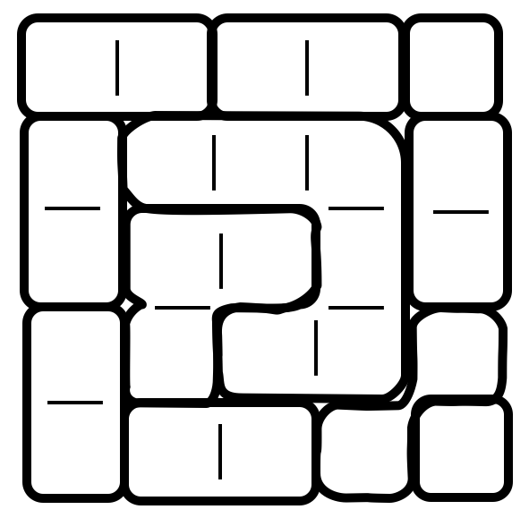
When we want to model this problem, we basically have three sets of constraints:
- Each row \(i\) has unique values \(1,\dots,5\)
- Each column \(j\) has unique values \(1,\dots,5\)
- Each region \(r\) has unique sums
This leads to repeated use of the all-different constraint.
Below I will try to model this problem in different ways:
- A MIP formulation using GAMS. When using integer programming we don't have an all-different construct. However, with a little bit of effort, we can implement this using linear constraints.
- A Python implementation using the Z3 SMT solver from Microsoft.
- A Minizinc implementation using the Gecode constraint programming solver.
The last two approaches allow us to use all-different directly.
In addition, I will discuss how we can verify that there there is only one unique solution to this problem.
MIP Model
As usual we will use a binary variable [2]: \[x_{i,j,k} = \begin{cases} 1 & \text{if cell $(i,j)$ has value $k$}\\ 0 & \text{otherwise}\end{cases}\]
Using this definition, the row and column uniqueness constraints are easy using assignment constraints: \[\begin{align} & \sum_i x_{i,j,k} = 1 & \forall j,k \\ & \sum_j x_{i,j,k} = 1 & \forall i,k \\ &\sum_k x_{i,j,k} = 1 &\forall i,j\end{align}\] These assignment constraint effectively implement what is known as all-different constraints in constraint programming. See [3] for different MIP formulations for these all-different constraints.
Let's indicate a region by \(r\). We can calculate the value of a region by: \[v_r = \sum_{(i,j)|R_{i,j,r}} \sum_k k\> x_{i,j,k} \] We sum over cells in region \(r\). Now we have to add an all-different constraint: \[\text{all-different}(v_k)\] This is a slightly different all-different constraint from the ones we discussed before. Here we don't enumerate all possible values.
One way to model this, is the following. Interpret the problem as: \[ v_r \le v_{r'} - 1 \textbf{ or } v_r \ge v_{r'} + 1 \>\> \forall r\ne r'\] We can model this with binary variables \(\delta\): \[\begin{align} & v_r \le v_{r'} - 1 + M\delta_{r,r'}\\ & v_r \ge v_{r'} + 1 -M (1-\delta_{r,r'})\\ & \delta_{r,r'} \in \{0,1\} \end{align}\] Instead of \(\forall r\ne r'\), we can save some equations and variables by only generating these constraints \(\forall i\lt j\). We need a good value for \(M\). If the largest possible value of a region is \(L\), then \(M=L+1\). The largest region has 6 cells, so one easy bound is \(L=6 \times 5=30\). With some more analysis we can reduce this even further, but I am happy with this bound.
Interestingly, we used in this model two different ways to implement all-different constraints.
GAMS Model: Mixed Integer Programming
The GAMS model can look like:
sets i 'rows'/r1*r5/ j 'columns'/c1*c5/ k 'values'/1*5/ r 'regions'/r1*r11/ ; table grid(i,j) 'encoding of regions' c1 c2 c3 c4 c5 r1 1 1 2 2 3 r2 4 5 5 5 6 r3 4 7 7 5 6 r4 8 7 5 5 10 r5 8 9 9 10 11 ; set region(i,j,r) '(i,j) is in r'; region(i,j,r) = grid(i,j) = ord(r); alias(r,r1,r2); set rr(r1,r2) 'compare r1,r2'; rr(r1,r2) = ord(r1)<ord(r2); parameter len(r) 'length of a region'; len(r) = sum(region(i,j,r),1); scalar M '1+largest value of a region'; M = 1+smax(r,len(r)) * card(k); display M; binaryvariables x(i,j,k) 'assign value k to cell (i,j)' delta(r1,r2) 'used to model OR constraint' ; variables v(r) 'value of a region' z 'dummy objective' ; equations value(i,j) 'unique value in cell' row(i,k) 'unique value in row' column(j,k) 'unique value in column' sumregion(r) 'sum of cell values in region' alldiff1(r1,r2) 'all-different constraint' alldiff2(r1,r2) 'all-different constraint' objective 'dummy objective' ; * * assignment constraints * value(i,j).. sum(k, x(i,j,k)) =e= 1; row(i,k).. sum(j, x(i,j,k)) =e= 1; column(j,k).. sum(i, x(i,j,k)) =e= 1; * * region values * sumregion(r).. v(r) =e= sum((region(i,j,r),k), x(i,j,k) * k.val); * * all-different(v) * alldiff1(rr(r1,r2)).. v(r1) =l= v(r2) - 1 + M*delta(r1,r2); alldiff2(rr(r1,r2)).. v(r1) =g= v(r2) + 1 - M*(1-delta(r1,r2)); * * dummy objective * objective.. z =e= 0; model m1 /all/; solve m1 minimizing z using mip; * * reporting * parameter xv(i,j) 'cell values'; xv(i,j) = sum(k, x.l(i,j,k) * k.val); option grid:0,xv:0,v:0; display grid,xv,v.l; |
The results look like:
----     88 PARAMETER grid  encoding of regions

            c1          c2          c3          c4          c5

r1           11223
r2           45556
r3           47756
r4           875510
r5           8991011


----     88 PARAMETER xv  cell values

            c1          c2          c3          c4          c5

r1           13542
r2           51423
r3           35214
r4           24135
r5           42351


----     88 VARIABLE v.L  value of a region

r1   4,    r2   9,    r3   2,    r4   8,    r5  12,    r6   7,    r7  11
r8   6,    r9   5,    r10 10,    r11  1
After playing with my crayons, we have:

This is not a super easy model to solve. Standard Sudoku models are typically solved in the presolve phase, so the MIP solver does not have to any branching. This is not the case with this model:
        Nodes                                         Cuts/
   Node  Left     Objective  IInf  Best Integer    Best Bound    ItCnt     Gap

000.0000610.000099
000.00002                     Cuts: 2101
000.00003                     Cuts: 6106
000.00003                 ZeroHalf: 2108
020.000030.0000108
Elapsed time = 0.25 sec. (25.37 ticks, tree = 0.01 MB, solutions = 0)
13381590.000030.000013389
                                                      Cuts: 8
2012123    infeasible                            0.000024769
282296    infeasible                            0.000038178
3072930.0000670.000042948
34861070.0000380.000050692
                                                     Cuts: 10
39091230.0000550.000059355
40401300.0000450.000062204
4150390.0000680.000064390
*  42340      integral     00.00000.0000661840.00%
Found incumbent of value 0.000000 after 9.97 sec. (2491.49 ticks)
The solver has to do some real work here: 4234 nodes and 66184 simplex iterations. As this is a feasibility problem, we can stop as soon as we find a feasible integer solution.
Uniqueness of the solution
It is easy to add a constraint that checks the uniqueness of this solution. Let's first record the current solution: \(a_{i,j,k} = x^*_{i,j,k}\). Now add the constraint:\[\sum_{i,j,k} a_{i,j,k} x_{i,j,k} \le 5^2-1\] Solve this model and check the status. If this new problem is infeasible, we know our original solution was unique.
When I did this the solver showed:
MIP status(119): integer infeasible or unbounded
In general, I find this always a bit a of disappointing message. The solver should be able to make up its mind (even if it takes a few micro-seconds: the user's time is really more important than a little bit of computation time for the solver).
In this case it is even more troubling. The model has a dummy objective \(z=0\). So if the solver says, well, may be the model is unbounded, it clearly was not paying attention.
Constraint solver: Z3/Python
A constraint solver typically has built-in support for the all-different constraint. This allows us to use \(x_{i,j} \in 1,\dots,5\) directly as main variable. A Z3 python model can look like:
from z3 import *

grid = [[ 1,   1,   2,   2,   3],
        [ 4,   5,   5,   5,   6],
        [ 4,   7,   7,   5,   6],
        [ 8,   7,   5,   5,  10],
        [ 8,   9,   9,  10,  11]]


ROWS = range(len(grid))     # 0..rows-1
COLS = range(len(grid[0]))  # 0..cols-1
MAX = 5# 1 <= x[i,j] <= MAX

REGIONS = set([grid[i][j] for i in ROWS for j in COLS])  # region numbers

# for each region form a list of (i,j) tuples
region = [[] for r in REGIONS]
for i in ROWS:
for j in COLS:
        r = grid[i][j]
        region[r-1] += [(i,j)]

#
# decision variables
#
X = [ [ Int("x%d.%d" % (i+1, j+1)) for j in COLS ] for i in ROWS ]
V = [ Int("v%d" % r) for r in REGIONS]

#
# constraints
#
Bounds = And([And(X[i][j] >= 1,X[i][j] <= MAX) for i in ROWS for j in COLS ])
UniqRows = And([ Distinct([X[i][j] for j in COLS]) for i in ROWS])
UniqCols = And([ Distinct([X[i][j] for i in ROWS]) for j in COLS])
UniqRegionValues = Distinct([V[r-1] for r in REGIONS])
CalcV = And([V[r-1] == Sum([X[i][j] for (i,j) in region[r-1]]) for r in REGIONS])

Cons = [Bounds, UniqRows, UniqCols, UniqRegionValues, CalcV]

#
# solve and print solution
#
s = Solver()
s.add(Cons)
if s.check() == sat:
     m = s.model()
     sol = [ [ m.evaluate(X[i][j]) for j in COLS] for i in ROWS]
print(sol)

#
# Check for uniqueness
#
Forbid = Or([X[i][j] != sol[i][j] for i in ROWS for j in COLS])
s.add(Forbid)
if s.check() == sat:
print("There is an alternative solution.")
else:
print("Solution is unique.")
The output looks like:
[[1, 3, 5, 4, 2], [5, 1, 4, 2, 3], [3, 5, 2, 1, 4], [2, 4, 1, 3, 5], [4, 2, 3, 5, 1]]
Solution is unique.
In this model I tried to be efficient w.r.t constraint Calcv. Basically I tried to make only one pass over the data grid[i][j]. As this model is small, I probably could have dropped the calculation of region and immediate form the equation:
CalcV = And([V[r-1] == Sum([X[i][j] for i in COLS for j in ROWS if grid[i][j] == r]) for r in REGIONS])
This will make multiple passes over grid[i][j], but that is not a problem for a model with this size.
Constraint solver: Minizinc/Gecode
This model can be coded easily in Minizinc:
include "globals.mzn";

% number of rows, columns, regions
int: m = 5;
int: n = 5;
int: nr = 11;

% sets
set of int: I = 1..m;
set of int: J = 1..n;
set of int: R = 1..nr;

% grid
array[I,J] of int: grid;
grid = [| 1,   1,   2,   2,   3,
        | 4,   5,   5,   5,   6,
        | 4,   7,   7,   5,   6,
        | 8,   7,   5,   5,  10,
        | 8,   9,   9,  10,  11  |];


array[I,J] of var int: x;
array[R] of var int: v;

constraint forall (i in I, j in J) ( x[i,j] >= 1 );

constraint forall (i in I, j in J) ( x[i,j] <= 5 );

constraint forall (i in I) ( alldifferent([ x[i,j] | j in J]) );

constraint forall (j in J) ( alldifferent([ x[i,j] | i in I]) );

constraint forall (r in R) ( v[r] = sum( [ x[i,j] | i in I, j in J where grid[i,j] = r] ) );

constraint alldifferent( [v[r] | r in R] );

solve satisfy;
I did not optimize the constraint that calculates v[r]. I assume this version will make multiple passes over grid[i,j].
Gecode will try to find multiple solutions, but it finds just one:
Compiling sudokux.mzn
Running sudokux.mzn
x = array2d(1..5 ,1..5 ,[1, 3, 5, 4, 2, 5, 1, 4, 2, 3, 3, 5, 2, 1, 4, 2, 4, 1, 3, 5, 4, 2, 3, 5, 1]);
v = array1d(1..11 ,[4, 9, 2, 8, 12, 7, 11, 6, 5, 10, 1]);
----------
==========
Finished in 333msec
Minizinc does not know how to print tables so unfortunately we get the results as a long list. It is possible to do your own formatting, but it strange that the default behavior is so user unfriendly. A better layout would really help.
Performance
This is not a very easy model. Here are some timings:
| Model | Solver | Solution Time | Nodes | Iterations | Notes |
|---|---|---|---|---|---|
| MIP | Cplex | 9.97 | 4234 | 66184 | 1 thread |
| MIP | CBC | 276 | 158405 | 3192290 | |
| Constraint | Z3 | 37.5 | |||
| Constraint | Gecode | 0.333 |
We see quite a variation in solution times. This is not unusual for combinatorial problems like this.
References
- https://blogs.wsj.com/puzzle/2018/05/24/varsity-math-week-141/ and https://momath.org/home/varsity-math/varsity-math-week-141/
- https://yetanothermathprogrammingconsultant.blogspot.com/2016/10/mip-modeling-from-sudoku-to-kenken.html
- Williams, H. Paul and Yan, Hong (2001), Representations of the 'all_different' predicate of constraint satisfaction in integer programming, Informs Journal on Computing, 13 (2). 96-103.