Rectangular Covering
This problem is from [1].
Problem statement: given \(N\) data points, arrange \(k\) boxes such that every point is inside a box and the size of the boxes is minimized. We assume the boxes have sides parallel to the axes. I.e. the box is not angled.
A 2d data set with \(N=50\) points can look like:
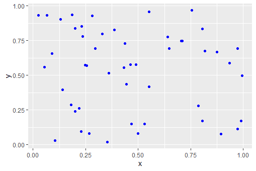 |
| N=50 data points |
The best configuration of \(K=5\) boxes for this data set is:
 |
| Optimal solution for K=5 rectangles |
The problem is a like the opposite of the "largest empty box" [2], where we try to find the largest box without any data points inside.
2D Model
Let's define some symbols:
A high-level model for 2 dimensions can look like:
- We will denote the data points by \(i\) and the rectangles by \(k\).
- The coordinates of the data points are stored in \(p_{i,c} \in [L,U]\) with \(c \in \{x,y\}\).
- The location and size of the rectangles are \(r_{k,s}\in [L,U]\) . Here \(s\in \{x,y,w,h\}\).
- The assignment of (data) points to rectangles is modeled with a binary variable \(x_{i,k} \in \{0,1\}\).
A high-level model for 2 dimensions can look like:
| High-level 2D MIQP model |
|---|
| \[\begin{align}\min & \sum_k \color{darkred} r_{k,w} \cdot \color{darkred} r_{k,h} \\ & \sum_k \color{darkred}x_{i,k} = 1 && \forall i \\ & \color{darkred}x_{i,k}=1 \implies \begin{cases} \color{darkblue}p_{i,x} \ge \color{darkred}r_{k,x} \\ \color{darkblue}p_{i,y} \ge \color{darkred}r_{k,y} \\ \color{darkblue}p_{i,x} \le \color{darkred}r_{k,x}+\color{darkred}r_{k,w} \\ \color{darkblue}p_{i,y} \le \color{darkred}r_{k,y}+\color{darkred}r_{k,h} \end{cases} && \forall i,k\\ & \color{darkred} x_{i,k}\in \{0,1\} \\ & \color{darkred}r_{k,h} \in [\color{darkblue}L,\color{darkblue}U] \\ &\color{darkred}r_{k,x}+\color{darkred}r_{k,w} \le \color{darkblue}U \\ &\color{darkred}r_{k,y}+\color{darkred}r_{k,h} \le \color{darkblue}U \end{align}\] |
The implication says "if \(x_{i,k}=1\) then point \(i\) should be in box \(k\)". This can be implemented using indicator constraints or with a big-M construct: \[\begin{align} & p_{i,x} \ge r_{k,x} -M(1-x_{i,k})\\ & p_{i,y} \ge r_{k,y}-M(1-x_{i,k}) \\ & p_{i,x} \le r_{k,x}+r_{k,w} +M(1-x_{i,k})\\ & p_{i,y} \le r_{k,y}+r_{k,h}-M(1-x_{i,k}) \end{align}\] A value for \(M\) can be \(M=U-L\). We can of course scale the data \(p_{i,c}\) to \(p_{i,c} \in [0,1]\) beforehand, in which case we can set \(M=1\). This is what I did in my experiments.
I also add the constraint: \[r_{k,x} \ge r_{k-1,x}\] to make the solution more predictable. The solution will be ordered by the \(x\)-coordinate of the box. It also reduces symmetry in the model.
The objective has non-convex quadratic terms. So we need a non-convex quadratic solver.
The detailed data and solution look like:
----     56 PARAMETER p  data points

              x           y

i1      0.806010.17283
i2      0.529520.14887
i3      0.648260.69240
i4      0.352220.02016
i5      0.431300.55356
i6      0.640870.77456
i7      0.235450.78074
i8      0.268000.08158
i9      0.973280.11440
i10     0.874310.66711
i11     0.756210.96771
i12     0.198630.24001
i13     0.219900.26101
i14     0.988630.17156
i15     0.066250.93008
i16     0.806030.83235
i17     0.105430.02902
i18     0.229270.09355
i19     0.129830.90322
i20     0.436820.72756
i21     0.247540.57512
i22     0.360120.51628
i23     0.710150.74601
i24     0.703670.74621
i25     0.185170.93583
i26     0.816810.67338
i27     0.463500.57754
i28     0.089320.65688
i29     0.973350.69059
i30     0.894490.07780
i31     0.141240.39550
i32     0.993820.49870
i33     0.054060.56047
i34     0.329270.79803
i35     0.229750.85134
i36     0.785320.27930
i37     0.180140.28874
i38     0.386280.82680
i39     0.489700.57654
i40     0.467090.14913
i41     0.199490.83893
i42     0.254380.57046
i43     0.551160.95672
i44     0.026340.93260
i45     0.499500.08040
i46     0.445290.43742
i47     0.551000.41666
i48     0.296260.69398
i49     0.934260.58556
i50     0.280830.92941


----     56 VARIABLE x.L  assignment variables

             k1          k2          k3          k4          k5

i1                                                      1.00000
i2                              1.00000
i3      1.00000
i4                              1.00000
i5                                          1.00000
i6      1.00000
i7      1.00000
i8                              1.00000
i9                                                      1.00000
i10                                                     1.00000
i11     1.00000
i12                 1.00000
i13                 1.00000
i14                                                     1.00000
i15     1.00000
i16     1.00000
i17                             1.00000
i18                             1.00000
i19     1.00000
i20     1.00000
i21                 1.00000
i22                                         1.00000
i23     1.00000
i24     1.00000
i25     1.00000
i26                                                     1.00000
i27                                         1.00000
i28                 1.00000
i29                                                     1.00000
i30                                                     1.00000
i31                 1.00000
i32                                                     1.00000
i33                 1.00000
i34     1.00000
i35     1.00000
i36                                                     1.00000
i37                 1.00000
i38     1.00000
i39                                         1.00000
i40                             1.00000
i41     1.00000
i42                 1.00000
i43     1.00000
i44     1.00000
i45                             1.00000
i46                                         1.00000
i47                                         1.00000
i48     1.00000
i49                                                     1.00000
i50     1.00000


----     56 VARIABLE r.L  rectangles

             x           y           w           h

k1     0.026340.692400.779690.27530
k2     0.054060.240010.200320.41687
k3     0.105430.020160.424090.12897
k4     0.360120.416660.190870.16088
k5     0.785320.077800.208500.61279


----     56 VARIABLE z.L                   =      0.51132  objective
This model was solved to proven global optimality with Gurobi in about 670 seconds.
To higher dimensions
The above model dealt with the 2D problem. It is not very difficult to extend this to more dimensions. Let's try to make this general, for any dimension.
First of all, I reorganized my sets a bit:
- We have \(d \in \{1,\dots,D\}\) indicating the dimension we are looking at. Think about this as \(1=x,2=y,3=z,...\).
- To characterize a box, for each dimension, we have a coordinate and a side-length. So, \(cs \in \{\mathrm{coord},\mathrm{side}\}\).
With this, we can write:
- \(p_{i,d}\) are the coordinates of the points,
- \(r_{k,d,cs}\) indicate the location and size of the boxes.
The model can now look like:
| High-level n-dimensional MINLP model |
|---|
| \[\begin{align}\min & \sum_k \prod_d \color{darkred} r_{k,d,side} \\ & \sum_k \color{darkred}x_{i,k} = 1 && \forall i \\ & \color{darkred}x_{i,k}=1 \implies \begin{cases} \color{darkblue}p_{i,d} \ge \color{darkred}r_{k,d,coord} \\ \color{darkblue}p_{i,d} \le \color{darkred}r_{k,d,coord}+\color{darkred}r_{k,d,side} \end{cases} && \forall i,k,d\\ & \color{darkred} x_{i,k}\in \{0,1\} \\ & \color{darkred}r_{k,d,cs} \in [\color{darkblue}L,\color{darkblue}U] \\ &\color{darkred}r_{k,d,coord}+\color{darkred}r_{k,d,side} \le \color{darkblue}U \end{align}\] |
The objective is not quadratic. We can make it quadratic by chaining[2]. We introduce a variable \(v\) which is defined by:\[v_{k,d} = \begin{cases} v_{k,d-1}\cdot r_{k,d,side} & \text{for $d\ge 2$}\\ 1 & \text{for $d=1$}\end{cases}\] Now we can just minimize \(\sum_k v_{k,D}\). For the special case of a 3d problem, we can simplify this to: \[\begin{align} \min & \sum_k \mathit{area}_k \cdot r_{k,3,side} \\ & \mathit{area}_k = r_{k,1,side}\cdot r_{k,2,side}\end{align}\]
This is a rather difficult model for Gurobi. I tried with the following 3d data set:
----     17 PARAMETER p  data points

           dim1        dim2        dim3

i1      0.806010.172830.52952
i2      0.148870.648260.69240
i3      0.352220.020160.43130
i4      0.553560.640870.77456
i5      0.235450.780740.26800
i6      0.081580.973280.11440
i7      0.874310.667110.75621
i8      0.967710.198630.24001
i9      0.219900.261010.98863
i10     0.171560.066250.93008
i11     0.806030.832350.10543
i12     0.029020.229270.09355
i13     0.129830.903220.43682
i14     0.727560.247540.57512
i15     0.360120.516280.71015
i16     0.746010.703670.74621
i17     0.185170.935830.81681
i18     0.673380.463500.57754
i19     0.089320.656880.97335
i20     0.690590.894490.07780
i21     0.141240.395500.99382
i22     0.498700.054060.56047
i23     0.329270.798030.22975
i24     0.851340.785320.27930
i25     0.180140.288740.38628
i26     0.826800.489700.57654
i27     0.467090.149130.19949
i28     0.838930.254380.57046
i29     0.551160.956720.02634
i30     0.932600.499500.08040
i31     0.445290.437420.55100
i32     0.416660.296260.69398
i33     0.934260.585560.28083
i34     0.929410.478000.62209
i35     0.772930.070780.06152
i36     0.149700.917170.49579
i37     0.378920.849310.39839
i38     0.546640.615100.73048
i39     0.513430.392460.82100
i40     0.624360.539450.24515
i41     0.374560.961790.50185
i42     0.074250.428490.98776
i43     0.639380.806350.03245
i44     0.903470.127140.86304
i45     0.739780.973460.25849
i46     0.426700.075500.16401
i47     0.564370.748780.57450
i48     0.369460.959250.80891
i49     0.185910.367490.29618
i50     0.155500.422850.79756
and \(K=5\) boxes. Gurobi was able to find some integer solutions within one hour of computation time, but the gap was still very large (40%). The results looked like:
----    107 VARIABLE x.L  assignment variables

             k1          k2          k3          k4          k5

i1                                                            1
i2                        1
i3                                                1
i4                                                            1
i5                                    1
i6                                    1
i7                                                            1
i8            1
i9                        1
i10                       1
i11                                   1
i12           1
i13                       1
i14                                                           1
i15                                               1
i16                                                           1
i17                       1
i18                                                           1
i19                       1
i20                                   1
i21                       1
i22                                                           1
i23                                   1
i24                                   1
i25                       1
i26                                                           1
i27           1
i28                                                           1
i29                                   1
i30                                   1
i31                                                           1
i32                                                           1
i33                                   1
i34                                                           1
i35           1
i36                       1
i37                                               1
i38                                                           1
i39                                                           1
i40                                   1
i41                                               1
i42                       1
i43                                   1
i44                                                           1
i45                                   1
i46           1
i47                                                           1
i48                                               1
i49                       1
i50                       1


----    107 VARIABLE r.L  rectangles

    dim1.coord   dim1.side  dim2.coord   dim2.side  dim3.coord   dim3.side

k1      0.02900.93870.07080.15850.06150.1785
k2      0.07420.14570.06630.86960.29620.6976
k3      0.08160.85270.49950.47400.02630.2545
k4      0.35220.02670.02020.94160.39840.4105
k5      0.41670.51270.05410.69470.52950.3335


----    107 VARIABLE z.L                   =       0.3469  objective
References
- How can I find k minimum bounding rectangles to enclose all the given points?, https://stackoverflow.com/questions/60401171/how-can-i-find-k-minimum-bounding-rectangles-to-enclose-all-the-given-points
- Non-convex Quadratic Models, http://yetanothermathprogrammingconsultant.blogspot.com/2020/02/non-convex-quadratic-models.html