In Statistics (nowadays called Data Science or A.I. for public relations reasons), clustering is one of the most popular techniques available. Of course, nothing beats linear regression. Here, I like to discuss two models: \(k\)-means and \(k\)-medoids. For these models, there are equivalent Mixed-Integer Programming models. In practice, they don't work very well except for small data sets. I think they are still useful to discuss for different reasons:
- The formulations are interesting. They have some angles that may not be obvious at first.
- They define the model in a succinct way. Verbal descriptions are always fraught with imprecision and vagueness. A reference model can help to make things explicit.
- Not all data sets are large. For small data sets, we can prove optimality where the usual heuristics only can deliver good solutions, without much information about the quality of the solution. Obviously, clustering is often used in situations where ultimate optimality may not matter much, as it is frequently used as an exploratory tool.
- We can adapt the model to special cases. Adding constraints such as a minimum and maximum number of points per cluster comes to mind [3].
K-means clustering
\(k\)-means clustering is an immensely popular technique to make some sense from highly-dimensional data. The term \(k\)-means was introduced in 1967 [2] described as a way "a process for partitioning an \(N\)-dimensional population into \(k\) sets on the basis of a sample". The number of clusters \(k\) is determined beforehand. The method will minimize the within-cluster sum-of-squares between the points and the centroid of the cluster. Our model has two variables:
- \(\color{darkred}x_{i,k}\in\{0,1\}\) indicates the assignment of points \(\color{darkblue}p_i\) to clusters \(k\) and
- \(\color{darkred}\mu_{k,c}\): the coordinates of the centroid of cluster \(k\). The index \(c\) indicates the coordinates or features.
The centroids can be calculated by simply averaging the points in each cluster. Note that this is non-linear as the number of points in a cluster is not constant, but variable. However, we do not need to explicitly calculate the means: just by minimizing the squared distances, we obtain automatically the correct value for \(\color{darkred}\mu_k\). The centroids are minimizers of the within-cluster sum-of-squares. This is exactly what we are optimizing. So here is a first model:
| Non-convex MINLP Model |
|---|
| \[\begin{align}\min&\sum_{i,k,c}\left(\color{darkblue}p_{i,c}-\color{darkred}\mu_{k,c}\right)^2 \cdot \color{darkred}x_{i,k}\\ &\sum_k \color{darkred}x_{i,k}=1&&\forall i \\&\color{darkred}x_{i,k}\in \{0,1\} \end{align}\] |
Here \(\color{darkblue}p_{i,c}\) is our data matrix. This model will simultaneously determine the optimal assignments \(\color{darkred}x\) and the centroids \(\color{darkred}\mu\).
We can convexify this model as follows:
| Convex MIQCP Model |
|---|
| \[\begin{align}\min&\sum_{i,k}\color{darkred}d_{i,k}\\ &\color{darkred}d_{i,k}\ge \sum_c\left(\color{darkblue}p_{i,c}-\color{darkred}\mu_{k,c}\right)^2-\color{darkblue}M\cdot(1- \color{darkred}x_{i,k})\\ &\sum_k \color{darkred}x_{i,k}=1&&\forall i \\&\color{darkred}x_{i,k}\in \{0,1\} \\ & \color{darkred}d_{i,k}\ge 0\end{align}\] |
The centroid is always inside the convex hull of the points \(\color{blue}p_{i,c}\). So we can add the bounds:\[\color{darkred}\mu_{k,c} \in [\min_i \color{darkblue}p_{i,c},\max_i \color{darkblue}p_{i,c}]\] The big-M constant can be set to \[\color{darkblue}M=\max_{i,i'}\sum_c\left(\color{darkblue}p_{i,c}-\color{darkblue}p_{i',c}\right)^2\]
Some results
----     84 PARAMETER clusters

              points         SoS       mu(x)       mu(y)      avg(x)      avg(y)

cluster1      16.00010273.09068.75551.76768.75551.767
cluster2      10.0003295.20717.62873.89317.62873.893
cluster3      14.0002955.08425.31318.93425.31318.934
total         40.00016523.380
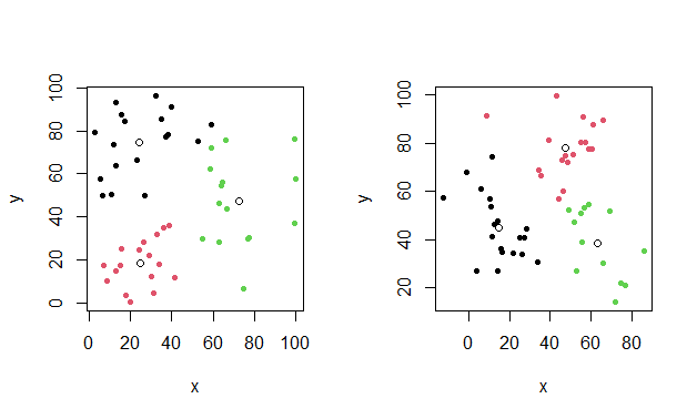
- rnd: generate 50 points with \(\color{darkblue}p_{i,c}\sim U(0,100)\)
- rclus: generate 50 points around 3 locations:\(\color{darkblue}p_{i,c}\sim N(L_{k,c},15)\) (standard deviation of 15).
- Without the ordering constraint
- With the ordering constraint
----    119 PARAMETER results

                   rnd     rnd+ord       rclus   rclus+ord

points          50.00050.00050.00050.000
clusters         3.0003.0003.0003.000
vars           310.000310.000310.000310.000
  discr        150.000150.000150.000150.000
equs           204.000206.000204.000206.000
status         Optimal     Optimal     Optimal     Optimal
obj          21104.16521104.16614736.05914736.059
time          2535.5781195.8441581.750254.093
nodes      1.541312E+76805599.0001.008025E+71802528.000
iterations 8.102010E+74.050808E+75.171027E+71.043268E+7
- MIQCP models are not suited for this problem: a model with just 150 binary variables takes way too long to find optimal solutions. The performance is really pathetic. Quadratic models can be really difficult for the current crop of high-end solvers.
- These results were with Cplex. Gurobi had even more troubles with these models.
- The ordering constraint can help a bit.
- Uniform random data makes things more difficult than data organized around some clusters.
- In the plots of the optimal clustering below, we don't see immediately much difference in the two data sets, but the MIQCP model does (according to the runtimes).
- There has been more success using column generation for this type of clustering [5].
 |
| k-means results with additional centroids |


K-medoids clustering
- The basic idea is to use as centers an actual point. This is opposed to \(k\)-means where we used a continuous variable \(\color{darkred}\mu_{k,c}\). In the \(k\)-medoid approach we pick as centers the point inside the cluster that minimizes the total within-cluster distances.
- As the center is a data point, we can easily interpret this point as being "representative" of a cluster.
- In the \(k\)-medoid problem we can calculate the distances in advance. This allows us to choose a distance metric. Typically one chooses the Euclidean distance or the Manhattan distance. Note that the \(k\)-means-method used the squared Euclidean distances.
- Manhattan distances (a.k.a. taxicab or L1 distances) are useful as they are more robust against outliers.
- As we will see, this model can be formulated as a MIQP or a linear MIP.
- We keep our assignment variable \(\color{darkred}x_{i,k}\) as before. The new definition of the center is: \[\color{darkred}\mu_{i,k} = \begin{cases} 1 & \text{if point $i$ is the center of cluster $k$} \\ 0 & \text{otherwise} \end{cases}\]
| Non-convex MIQP Model |
|---|
| \[\begin{align}\min&\sum_{i,i',k}\color{darkblue}d_{i,i'}\cdot \color{darkred}x_{i,k} \cdot \color{darkred}\mu_{i',k}\\ &\sum_k \color{darkred}x_{i,k}=1&&\forall i \\& \sum_i \color{darkred}\mu_{i,k}=1&&\forall k \\ &\color{darkred}\mu_{i,k} \le\color{darkred}x_{i,k} \\&\color{darkred}x_{i,k}\in \{0,1\}\\&\color{darkred}\mu_{i,k}\in \{0,1\} \end{align}\] |
Here \(\color{darkred}\mu\) is no longer the average, but a single point from the cluster. The distances \(\color{darkblue}d\) are calculated in advance. Like for \(k\)-means we may normalize the data first in case the units of the different features are different.
The first constraint in the model is the assignment constraint and is the same as in the \(k\)-means model. The second constraint says that there should be exactly one "center point" in each cluster. The third inequality constraint says that this center point has to be chosen from the points inside the cluster.
The model is easily linearized. Some solvers will do this automatically, or we can do this ourselves:
| Linear MIP Model |
|---|
| \[\begin{align}\min&\sum_{i,i',k}\color{darkblue}d_{i,i'}\cdot \color{darkred}y_{i,i',k} \\ &\color{darkred}y_{i,i',k} \ge \color{darkred}x_{i,k}+ \color{darkred}\mu_{i',k}-1 \\ &\sum_k \color{darkred}x_{i,k}=1&&\forall i \\& \sum_i \color{darkred}\mu_{i,k}=1&&\forall k \\ &\color{darkred}\mu_{i,k} \le\color{darkred}x_{i,k} \\&\color{darkred}x_{i,k}\in \{0,1\}\\&\color{darkred}\mu_{i,k}\in \{0,1\} \\ &\color{darkred}y_{i,i',k} \in [0,1] \end{align}\] |
Here \(\color{darkred}y\) can be continuous between 0 and 1 or binary (some solvers will make it binary automatically).
As before we can add an ordering constraint. Here I ordered on the number of points in the cluster.
Some results
Here are some results (different solver and different machine than for the \(k\)-means results):
----    140 PARAMETER results

                   rnd     rnd+ord       rclus   rclus+ord

points          50.00050.00050.00050.000
clusters         3.0003.0003.0003.000
vars           304.000304.000304.000304.000
  discr        300.000300.000300.000300.000
equs            57.00059.00057.00059.000
status         Optimal     Optimal     Optimal     Optimal
obj            937.013937.013821.179821.179
time             7.03215.3708.27016.324
nodes         1220.0001249.0001127.0001219.000
iterations   13539.00035659.00023242.00031547.000
This linarized MIQP model solves very fast with Gurobi. Cplex had extreme problems with this model. Incredibly, for the \(k\)-means problems, Cplex is much faster than Gurobi.
Here the ordering constraint does not really help.
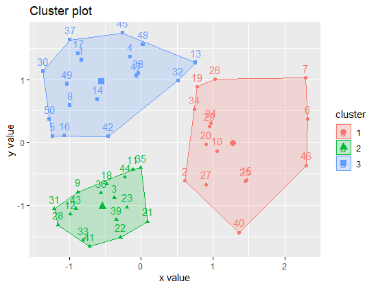
In R, we can use the pam function from the cluster package. It uses a heuristic, and, similar to kmeans, we can run it several times to prevent being stuck in a bad local minimum. In case you are wondering: PAM stands for Partitioning Around Medoids.
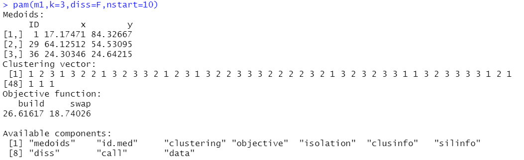
The objective 18.74026 seems not the same as I found (937.013). The reason is that pam reports as objective the average distance. So we need to compare 50 times 18.74026 to our 937.013, which is the same.
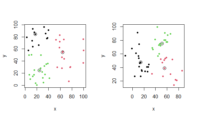 |
| k-medoids results with selected medoids |
Conclusions
The heuristics implemented in the kmeans and pam functions in R are far more efficient than using an MIQCP or MIP solver. We can use the optimization models as a "reference implementation", or for special cases.
I will probably never use these models on practical large data sets, but playing with these models (and writing things down), I have gained some useful insights and experience with clustering models. I think I know a bit more about clustering than before. So the main lesson: even useless optimization models are useful.
References
- \(K\)-means clustering, https://en.wikipedia.org/wiki/K-means_clustering
- MacQueen, J. B. (1967). Some Methods for classification and Analysis of Multivariate Observations. Proceedings of 5th Berkeley Symposium on Mathematical Statistics and Probability. 1. University of California Press. pp. 281–297.
- Any Solution for k-means with minimum and maximum cluster size constraint? https://or.stackexchange.com/questions/6227/any-solution-for-k-means-with-minimum-and-maximum-cluster-size-constraint
- \(K\)-medoids, https://en.wikipedia.org/wiki/K-medoids
- Aloise, D., Hansen, P. & Liberti, L. An improved column generation algorithm for minimum sum-of-squares clustering. Math. Program. 131, 195–220 (2012)