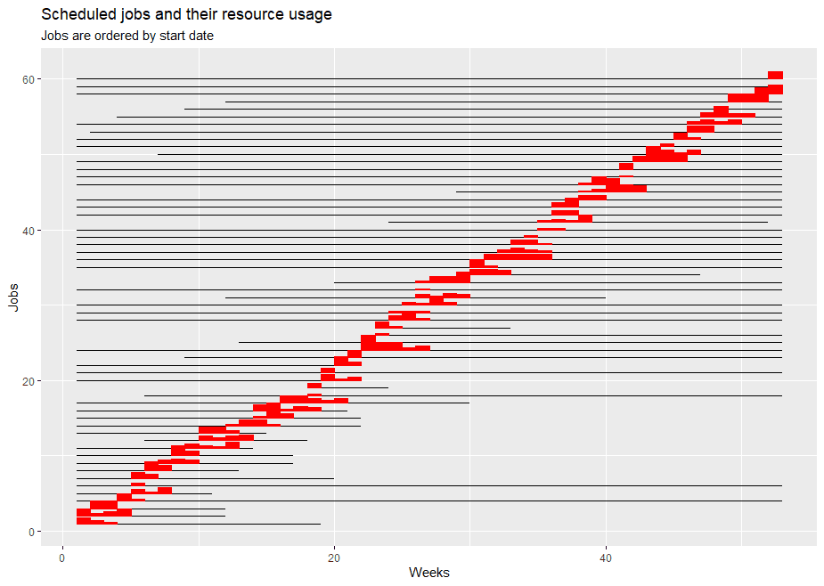
A scheduling problem: a modeling approach

Here is a simple scheduling problem [1]:

We have $T$ time periods (weeks)
and $N$ jobs to be scheduled.
Each job has a duration or processing time (again expressed in weeks), and a given resource (personnel) requirement during the execution of the job. This demand is expressed as: $\color{darkblue}{\mathit{resource}}_{j,t}$ where $j$ indicates the job and $t$ indicates the week since the start of the job.
Not in [1], but I added them to make things a bit more realistic: we have some release dates indicating that a job may not start before a given date. A reason can be that raw material is not available before that date.
Similarly, I added due dates: a job must finish before a given date.
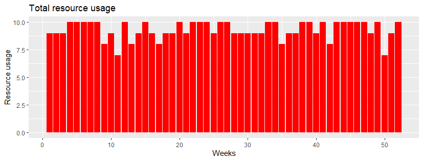
The objective is to minimize the maximum amount of resources we need over the whole planning period. We can think of this as the capacity we need (e.g. number of personnel).

In this post, I want to show a standard approach to model this problem and opposed to that, how I would attack this.

Data

It always helps to first look at some data. Here is my (random) data set:

----     32 SET jjobs

job1 ,    job2 ,    job3 ,    job4 ,    job5 ,    job6 ,    job7 ,    job8 ,    job9 ,    job10,    job11,    job12
job13,    job14,    job15,    job16,    job17,    job18,    job19,    job20,    job21,    job22,    job23,    job24
job25,    job26,    job27,    job28,    job29,    job30,    job31,    job32,    job33,    job34,    job35,    job36
job37,    job38,    job39,    job40,    job41,    job42,    job43,    job44,    job45,    job46,    job47,    job48
job49,    job50,    job51,    job52,    job53,    job54,    job55,    job56,    job57,    job58,    job59,    job60


----     32 SET tweeks

week1 ,    week2 ,    week3 ,    week4 ,    week5 ,    week6 ,    week7 ,    week8 ,    week9 ,    week10,    week11
week12,    week13,    week14,    week15,    week16,    week17,    week18,    week19,    week20,    week21,    week22
week23,    week24,    week25,    week26,    week27,    week28,    week29,    week30,    week31,    week32,    week33
week34,    week35,    week36,    week37,    week38,    week39,    week40,    week41,    week42,    week43,    week44
week45,    week46,    week47,    week48,    week49,    week50,    week51,    week52


----     32 PARAMETER data  job data and resource usage

          release         due    proctime       week1       week2       week3       week4       week5

job1            611
job2                       30555323
job3                       223143
job4            2244
job5                                    241
job6                       13254
job7                       12255
job8                                    544444
job9                                    11
job10                      113314
job11          29512554
job12                      223412
job13                                   555523
job14                      1741232
job15          2311
job16           745313
job17           912
job18                                   251
job19           61843234
job20                      193421
job21                      22252
job22                      17253
job23                                   11
job24                                   12
job25                                   3331
job26                      21545132
job27                                   251
job28                                   44555
job29                      1245235
job30          2333241
job31          182413
job32           13341
job33                                   12
job34                      14523214
job35                                   233
job36                                   244
job37                                   3154
job38                      2241441
job39          294742443
job40                                   3111
job41          123555
job42                                   15
job43                                   211
job44                                   13
job45           9215
job46          1315
job47          124042132
job48                                   3133
job49           443522
job50                                   234
job51                                   42152
job52          245241215
job53                                   42323
job54                      20243
job55                                   11
job56                                   11
job57                                   42321
job58                      153442
job59                                   14
job60          2041445

Notes:

The release date can be empty. That means we can start processing immediately on the corresponding job. Otherwise, we define the release date as the first week we can execute the job. In other words, the release date uses the beginning of the period. An empty release date can be interpreted as a release date of week 1.
The due date is also referring to the beginning of the period. If the due date is 4, we can still work on the job in week 3. An empty due date is the same as a due date of week 53.
The numbers under the week columns indicate the resource usage in that week (measured since the start of the job). Obviously, the length of the resource usage data is equal to the processing time or duration of the job.

An optimal solution can look like:

In this plot, the dark lines indicate the window between the release date and the due date. The red pieces are small bar charts indicating when jobs are executing and how many resources they consume. If we add up the red bars we get our final picture:

We have minimized the tallest bars in this plot.

Basic model

As usual, we start by defining our main decision variables. After that, things follow more or less automatically. So let's define: \[\color{darkred}x_{j,t} = \begin{cases}1 &\text{if job $j$ starts at time period $t$} \\ 0&\text{otherwise}\end{cases}\] Obviously, we need to start each job once, so we need something like \[\sum_t \color{darkred}x_{j,t} = 1 \>\>\forall t\] We know when a job starts at $t$, it will execute in $t'$ with $t' \in \{t,\dots,t+\color{darkblue}{\mathit{proctime}}_j-1\}$. This means that if we look at $t'$, the relevant jobs start at $t=t'-\color{darkblue}{\mathit{proctime}}_j+1,\dots,t'$. The capacity constraint now becomes: \[\color{darkblue}{\mathit{maxres}}\ge \sum_j \sum_{t=t'-\color{darkblue}{\mathit{proctime}}_j+1}^{t'} \color{darkblue}{\mathit{resource}}_{j,t'-t+1}\cdot \color{darkred}x_{j,t} \>\> \forall t'\] This construct uses a lot of index calculations, which makes the constraint difficult to read (and write). The release date constraint is simple: \[\sum_t t\cdot \color{darkred}x_{j,t}\ge\color{darkblue}{\mathit{release}}_{j} \>\> \forall j\] However, the due date also requires some index calculations: \[\sum_t (t+\color{darkblue}{\mathit{proctime}}_j-1)\cdot \color{darkred}x_{j,t}\le\color{darkblue}{\mathit{due}}_{j}-1 \>\> \forall j\] Instead of the release-date and due-date constraints we can also fix $\color{darkred}x_{j,t}=0$ when the index $t$ is outside the allowed range. That may be slightly simpler.

Here is a summary of this first model:

MIP Model 1
\[\begin{align}\min\>&\color{darkblue}{\mathit{maxres}} \\ & \sum_t \color{darkred}x_{j,t}=1 && \forall j \\ & \color{darkblue}{\mathit{maxres}}\ge \sum_j \sum_{t=t'-\color{darkblue}{\mathit{proctime}}_j+1}^{t'} \color{darkblue}{\mathit{resource}}_{j,t'-t+1}\cdot \color{darkred}x_{j,t} && \forall t' \\ & \sum_t t\cdot \color{darkred}x_{j,t}\ge\color{darkblue}{\mathit{release}}_{j} && \forall j\\ & \sum_t (t+\color{darkblue}{\mathit{proctime}}_j-1)\cdot \color{darkred}x_{j,t}\le\color{darkblue}{\mathit{due}}_{j}-1 && \forall j \\ & \color{darkred}x_{j,t} \in \{0,1\}\end{align}\]

MIP Model 1

\[\begin{align}\min\>&\color{darkblue}{\mathit{maxres}} \\ & \sum_t \color{darkred}x_{j,t}=1 && \forall j \\ & \color{darkblue}{\mathit{maxres}}\ge \sum_j \sum_{t=t'-\color{darkblue}{\mathit{proctime}}_j+1}^{t'} \color{darkblue}{\mathit{resource}}_{j,t'-t+1}\cdot \color{darkred}x_{j,t} && \forall t' \\ & \sum_t t\cdot \color{darkred}x_{j,t}\ge\color{darkblue}{\mathit{release}}_{j} && \forall j\\ & \sum_t (t+\color{darkblue}{\mathit{proctime}}_j-1)\cdot \color{darkred}x_{j,t}\le\color{darkblue}{\mathit{due}}_{j}-1 && \forall j \\ & \color{darkred}x_{j,t} \in \{0,1\}\end{align}\]

My model

I usually don't write models like the one presented in the previous paragraph. The index calculations in the constraints are too complex to write them down without making a few errors. My answer to that is to make the constraints simpler and precalculate sets and parameters in advance. The advantage of precalculating these is that we can debug them one by one before we have a running model. In addition, sets and parameters are easier to debug than equations.

The first parameter I developed is $\color{darkblue}{\mathit{resmap}}_{j,t,t'}$ (resource mapper) which indicates how many resources we need at time period $t'$ for job $j$ starting at $t$. This is a fairly large data structure. A partial view can look like:

----     88 PARAMETER resmap  resource mapper

                   week1       week2       week3       week4       week5       week6       week7       week8       week9

job1 .week6                                                                        1
job1 .week7                                                                                    1
job1 .week8                                                                                                1
job1 .week9                                                                                                            1
job2 .week1            55323
job2 .week2                        55323
job2 .week3                                    55323
job2 .week4                                                55323
job2 .week5                                                            55323
job2 .week6                                                                        5532
job2 .week7                                                                                    553
job2 .week8                                                                                                55
job2 .week9                                                                                                            5
job3 .week1            143
job3 .week2                        143
job3 .week3                                    143
job3 .week4                                                143
job3 .week5                                                            143
job3 .week6                                                                        143
job3 .week7                                                                                    143
job3 .week8                                                                                                14
job3 .week9                                                                                                            1
job4 .week2                        44
job4 .week3                                    44
job4 .week4                                                44
job4 .week5                                                            44
job4 .week6                                                                        44
job4 .week7                                                                                    44
job4 .week8                                                                                                44
job4 .week9                                                                                                            4
. . .

The indices on the left are the job id, $j$ and the week the job starts, $t$. The column headers are the weeks we are working on the job, $t'$.

The second data structure I created is a set $\color{darkblue}{\mathit{ok}}_{j,t}$ indicating which time slots are allowed for job $j$ to start. This can look like this (again a partial view):

----     93 SET okallowed slots for jobs to start

            week1       week2       week3       week4       week5       week6       week7       week8       week9

job1                                                                      YES         YES         YES         YES
job2          YES         YES         YES         YES         YES         YES         YES         YES         YES
job3          YES         YES         YES         YES         YES         YES         YES         YES         YES
job4                      YES         YES         YES         YES         YES         YES         YES         YES
job5          YES         YES         YES         YES         YES         YES         YES         YES         YES
job6          YES         YES         YES         YES         YES         YES         YES         YES         YES
job7          YES         YES         YES         YES         YES         YES         YES         YES         YES
job8          YES         YES         YES         YES         YES         YES         YES         YES         YES
job9          YES         YES         YES         YES         YES         YES         YES         YES         YES
job10         YES         YES         YES         YES         YES         YES         YES         YES
job12         YES         YES         YES         YES         YES         YES         YES         YES         YES
job13         YES         YES         YES         YES         YES         YES         YES         YES         YES
job14         YES         YES         YES         YES         YES         YES         YES         YES         YES
job16                                                                                 YES         YES         YES
job17                                                                                                         YES
job18         YES         YES         YES         YES         YES         YES         YES         YES         YES
job19                                                                     YES         YES         YES         YES
job20         YES         YES         YES         YES         YES         YES         YES         YES         YES
. . .

The second symbol $\color{darkblue}{\mathit{ok}}_{j,t}$ can be easily calculated from the parameter $\color{darkblue}{\mathit{resmap}}_{j,t,t'}$: basically just take the first two indices $(j,t)$. So, in a sense we just have to spent effort on one parameter.

After calculating these two symbols, I wrote the model as:

MIP Model 2
\[\begin{align}\min\>&\color{darkblue}{\mathit{maxres}} \\ & \sum_{t\|\color{darkblue}{\mathit{ok}}(j,t)} \color{darkred}x_{j,t}=1 && \forall j \\ & \color{darkred}{\mathit{use}}_{t'} = \sum_{j,t} \color{darkblue}{\mathit{resmap}}_{j,t,t'} \cdot \color{darkred}x_{j,t} && \forall t'\\ & \color{darkblue}{\mathit{maxres}}\ge \color{darkred}{\mathit{use}}_{t} && \forall t \\ & \color{darkred}x_{j,t} \in \{0,1\}\end{align}\]

MIP Model 2

\[\begin{align}\min\>&\color{darkblue}{\mathit{maxres}} \\ & \sum_{t|\color{darkblue}{\mathit{ok}}(j,t)} \color{darkred}x_{j,t}=1 && \forall j \\ & \color{darkred}{\mathit{use}}_{t'} = \sum_{j,t} \color{darkblue}{\mathit{resmap}}_{j,t,t'} \cdot \color{darkred}x_{j,t} && \forall t'\\ & \color{darkblue}{\mathit{maxres}}\ge \color{darkred}{\mathit{use}}_{t} && \forall t \\ & \color{darkred}x_{j,t} \in \{0,1\}\end{align}\]

Some remarks:

The constraints for the release and the due date have disappeared. These are now taken care of by the set $\color{darkblue}{\mathit{ok}}_{j,t}$ and the parameter $ \color{darkblue}{\mathit{resmap}}_{j,t,t'}$. We just never consider an $\color{darkred}x_{j,t}$ that is outside the allowed window.
That means our generated model is much smaller: fewer variables and fewer constraints.
I added a variable $\color{darkred}{\mathit{use}}_{t}$ indicating how many resources we need at each time period. This is not really needed but useful in reporting. Instead of recomputing this quantity during reporting, I added it to the model. Sometimes we add so-called "accounting rows" to models to compute quantities used for reporting. They are meant to make the solution easier to interpret.
Notice that our equations are much simpler and that much of the debugging has happened before we even wrote the first equation.

Results

The solution looks like:

----    140 VARIABLE x.L  start of job

            week1       week2       week4       week5       week6       week8      week10      week12      week14

job3                                                                                                            1
job6                                                            1
job7                        1
job10                                               1
job14                                                           1
job18                                   1
job19                                                                                   1
job20           1
job22                                                                       1
job26                                                                                                           1
job29           1
job33                                               1
job34                                                                       1
job38                                                                                               1
job54                                               1
job58                                                                                   1

    +      week16      week18      week19      week20      week22      week23      week24      week25      week26

job1                        1
job2            1
job12                                   1
job13                                                           1
job15                                                                       1
job21                                               1
job30                                                                       1
job31                       1
job32                                                                                   1
job40                                                                                   1
job44                                   1
job45                                               1
job46                                                           1
job47                                                                                                           1
job51                                                                                               1
job56                                                                                                           1
job60                                                                                                           1

    +      week29      week30      week31      week32      week33      week34      week35      week36      week37

job8                                    1
job23                                                                       1
job25                                                           1
job27                       1
job35                                                                                               1
job39           1
job43                                                                                   1
job48                                                                                                           1
job50                                                                                               1
job52                                                                                   1
job57                                               1

    +      week38      week41      week42      week43      week44      week45      week46      week47      week48

job4                                                                                    1
job5                                                                        1
job11           1
job16                                               1
job17                                                                                                           1
job24                                                           1
job28                                   1
job37           1
job49                                                                                               1
job53                                                                                   1
job55                       1
job59                       1

    +      week49      week51      week52

job9                                    1
job36                       1
job41           1
job42                                   1


----    140 VARIABLE use.L  resource usage

week1   9,    week2   9,    week3   9,    week4  10,    week5  10,    week6  10,    week7  10,    week8  10
week9   8,    week10  9,    week11  7,    week12 10,    week13  8,    week14  9,    week15 10,    week16  9
week17  8,    week18  9,    week19  9,    week20 10,    week21  9,    week22 10,    week23 10,    week24 10
week25  9,    week26 10,    week27 10,    week28  9,    week29  9,    week30  9,    week31  9,    week32  9
week33 10,    week34 10,    week35  8,    week36  9,    week37  9,    week38 10,    week39 10,    week40  9
week41 10,    week42  8,    week43 10,    week44 10,    week45 10,    week46 10,    week47 10,    week48  9
week49 10,    week50  7,    week51  9,    week52 10


----    140 VARIABLE maxres.L              =           10maximum resource usage

This is the same solution as was illustrated in the pictures earlier. Looking at the performance, the solver does not care much which formulation is used:

----    148 PARAMETER results  compare statistics

               model 1     model 2

vars          3121.0002178.000
  discr       3120.0002125.000
equs           232.000164.000
status         Optimal     Optimal
obj             10.00010.000
time             3.8754.312
iterations     617.000617.000

Obviously, the first model is bigger, but the presolver takes care of that. Note that this particular data set is extremely easy to solve (these models did not require any nodes). But just slightly different data may make this model much more difficult to solve to optimality.

Conclusion

In some scheduling models, we need to perform somewhat complicated index calculations. These can lead to complex equations that are difficult to write, read, debug and maintain. I prefer to move this complexity away from the constraints and into separate data steps. This allows us to debug complicated expressions in isolation.

As a side note: a possible disadvantage of our scheduling model is that it only looks at the largest resource usage. It does not care how wild the rest of the solution is. In practice, we may prefer some smoothness apart from the spikes.

References

Scheduling minimization Integer Programming problem formulation, https://or.stackexchange.com/questions/6606/scheduling-minimization-integer-programming-problem-formulation

Appendix: GAMS model

$ontext

   Scheduling minimization Integer Programming problem formulation
   https://or.stackexchange.com/questions/6606/scheduling-minimization-integer-programming-problem-formulation

$offtext

*---------------------------------------------------------------------------
* populate data set with random data
*---------------------------------------------------------------------------

set
dummy 'for prettier output'/release,due,proctime/
j 'jobs'/job1*job60/
t 'weeks'/week1*week52/
;

parameters
release(j)    'release date'
due(j)        'due date'
proctime(j)   'processing time (weeks)'
resource(j,t) 'resource usage'
;

proctime(j) = uniformint(1,5);
release(j)$(uniform(0,1)<=0.2) = uniformint(1,30);
due(j)$(uniform(0,1)<=0.3) = min(release(j)+proctime(j)+uniformint(5,25),card(t));
resource(j,t)$(ord(t)<=proctime(j)) = uniformint(1,5);

*---------------------------------------------------------------------------
* display data
*---------------------------------------------------------------------------

parameter data(j,*) 'job data and resource usage';
data(j,'release') = release(j);
data(j,'proctime') = proctime(j);
data(j,'due') = due(j);
data(j,t) = resource(j,t);
option data:0;
display j,t,data;

*---------------------------------------------------------------------------
* re-interpret empty due date
*---------------------------------------------------------------------------

due(j)$(due(j)=0) = card(t)+1;

*---------------------------------------------------------------------------
* reporting macros
*---------------------------------------------------------------------------

acronym TimeLimit, Optimal, Error;

parameter results(*,*) 'compare statistics';
$macro report(m,label) \
    results('vars',label) = m.numVar; \
    results(' discr',label) = m.numDVar; \
    results('equs',label) = m.numEqu; \
    results('status',label) = Error; \
    results('status',label)$(m.solvestat=1) = Optimal; \
    results('status',label)$(m.solvestat=3) = TimeLimit; \
    results('obj',label) = m.objval; \
    results('time',label) = m.resusd; \
    results('nodes',label) = m.nodusd; \
    results('iterations',label) = m.iterusd; \
    results('gap%',label)$(m.solvestat=3) = 100*abs(m.objest - m.objval)/abs(m.objest);   \
    display results;

*---------------------------------------------------------------------------
* model 1: formulation without precalculating data
*---------------------------------------------------------------------------

alias(t,tt);

binaryvariable x(j,t) 'start of job';
variable maxres 'maximum resource usage';

equation
   assign(j) 'a job can be started at one time'
   bound(t)   'maximum of resource usage'
   erelease(j) 'release date constraint'
   edue(j)     'due date constraint'
;

assign(j)..    sum(t, x(j,t)) =e= 1;
bound(tt)..    maxres =g= sum((j,t)$(ord(t)>=ord(tt)-proctime(j)+1 andord(t)<=ord(tt)), resource(j,tt-(ord(t)-1))*x(j,t));
erelease(j).. sum(t, ord(t)*x(j,t)) =g= release(j);
edue(j)..      sum(t, (ord(t)+proctime(j)-1)*x(j,t)) =l= due(j)-1;

model m1 /all/;
option optcr=0,threads=8;
solve m1 minimizing maxres using mip;

option x:0;
display maxres.l,x.l;

report(m1,"model 1")

*---------------------------------------------------------------------------
* precalculate sets/parameters resmap and ok.
*---------------------------------------------------------------------------

parameter resmap(j,t,tt) 'resource mapper';
resmap(j,t,tt)$(ord(t)>=release(j) andord(t)+proctime(j)<=due(j)) = resource(j,tt-(ord(t)-1));
option resmap:0;
display resmap;

set ok(j,t) 'allowed slots for jobs to start';
ok(j,t) = sum(tt$resmap(j,t,tt),1);
display ok;

*---------------------------------------------------------------------------
* model 2: formulation with precalculating data
*---------------------------------------------------------------------------

positivevariable use(t) 'resource usage';

equation
   assign2(j) 'a job can be started at one time'
   usage(tt) 'keep track of resource usage in each period'
   bound2(t) 'maximum of resource usage'
;

assign2(j).. sum(ok(j,t), x(j,t)) =e= 1;
usage(tt).. use(tt) =e= sum((j,t),resmap(j,t,tt)*x(j,t));
bound2(t).. maxres =g= use(t);

model m2 /all-m1/;
option optcr=0,threads=8;
solve m2 minimizing maxres using mip;

option x:0,use:0,maxres:0;
display x.l,use.l,maxres.l;

parameter solution(j,*) 'reporting';
solution(j,'release') = release(j);
solution(j,'proctime') = proctime(j);
solution(j,'due') = due(j);
solution(j,'start') = sum(t,ord(t)*x.l(j,t));
solution(j,'finish') = sum(t,(ord(t)+proctime(j)-1)*x.l(j,t));
option solution:0;
display solution;

report(m2,"model 2")

A scheduling problem: a modeling approach

Data

Basic model

My model

Results

Conclusion

References

Appendix: GAMS model

Trending Articles

Practice Sheet of Right form of verbs for HSC Students

Download: FK ft Shenky – Nakuyewa ”Prod by: Shenky”

How to win at Markstrat (Markstrat Tips and Tricks) – Vodites

Ominde Commission Report and Recommendations – Ominde Report of 1964

Bureau of Internal Revenue: Regional Offices (Directory)

GO 53 on Enhancement of Ex-gratia upto 5 Lakhs Toddy Tappers in Telangana

Cakewalk CA-2A Leveling Amplifier v2.0.1.97 WiN, v2.0.1.96 OSX Incl Keygen

Mp3 Download: Mdu - Kunjenjenjena

How the kill the job , when DTP request running for long hours.

Microsoft Intune から展開しているアプリのアップデートについて

18-year-old girl was beaten for half an hour by two Northampton men in 'an...

Car crash in Dunton Bassett leaves driver in critical condition

Macky 2, Two Others In Road Accident

Application log 00000000000000089514: Could not convert queue DLVST90CLNT

Detroit mafia: D’Anna Brothers agree to plea deal

Delivery block field greyed out using VA02

Muloraki Au

【個人撮影】スマホのプライベート映像♪「中に出さないで///」カラオケ屋での生ハメ撮りが流出ｗ【リベンジポルノ】＠PornHub

BREAKING NEWS: Diamond Platnumz Is Reported Dead After Ghastly Car Accident

FIAT 500 B0111 B0112