The MAX-CUT problem is quite famous [1]. It can be stated as follows:
Given an undirected graph \(G=(V,E)\), split the nodes into two sets. Maximize the number of edges that have one node in each set.
Here is an example using a random sparse graph:
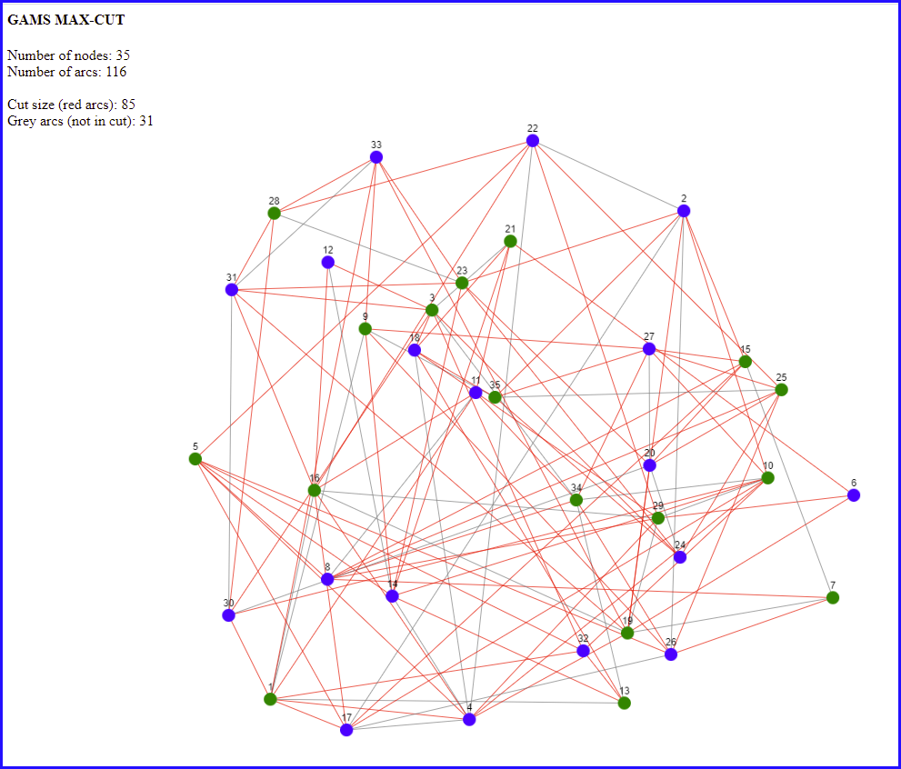 |
| MAX CUT, visualization using [2] |
Here we colored the two sets of nodes green and blue. We maximize the number of red arcs: they have a green and a blue node. The remaining arcs are grey. We see the optimal solution has a large number of red arcs.
There are some extensions:
- The graph can be sparse (as in the figure above): not every pair of nodes has an arc.
- We can use weights on the arcs and maximize the weighted sum of red arcs. We can think of the example as using weights \(\color{darkblue}w_{i,j}=1\). In this post I assume \(\color{darkblue}w_{i,j}\ge 0\).
- We can use a directed version: the maximum directed cut.
Max-Cut formulations
| Unconstrained quadratic model |
|---|
| \[\begin{align}\max&\sum_{(i,j)\in A} \color{darkblue}w_{i,j}\cdot \left(\color{darkred}x_i-\color{darkred}x_j \right)^2 \\ & \color{darkred}x_i\in\{0,1\} \end{align}\] |
Here \(A\) is the set of arcs. This is non-convex. However, a solver like Cplex will linearize this model automatically for us. We can see this in the log:
Classifier predicts products in MIQP should be linearized.
I.e. Cplex will solve this as a MIP instead of a non-convex MIQP.
We can force Cplex to solve as a quadratic model using the option qtolin=0. After this Cplex will automatically change the problem a bit to make it convex:
Repairing indefinite Q in the objective.
Instead of using a quadratic objective, we can also use slightly different objectives, such as: \[\max\>\sum_{(i,j)\in A} \color{darkblue}w_{i,j}\cdot \left| \color{darkred}x_i-\color{darkred}x_j \right|\] or \[\max\>\sum_{(i,j)\in A} \color{darkblue}w_{i,j}\cdot \left(\color{darkred}x_i \>{\bf xor }\> \color{darkred}x_j \right)\] Here \(\bf xor\) is the "exclusive or" operation, which can be defined by a truth table:
| \(x\) | \(y\) | \(x\>{\bf xor}\>y\) |
|---|---|---|
| 0 | 0 | 0 |
| 0 | 1 | 1 |
| 1 | 0 | 1 |
| 1 | 1 | 0 |
\(z =x\>{\bf xor}\>y\) can also be written as a system of linear inequalities: \[\begin{align}&z \le x+y\\ & z \ge x-y \\ & z \ge y-x \\ & z \le 2-x-y\end{align}\] As we are maximizing \(z\), we can drop the \(\ge\) conditions. Of course, we can also interpret the two included inequalities directly: \[\begin{align} & z \le x+y: && x=y=0 \Rightarrow z=0 \\ & z \le 2-x-y: && x=y=1 \Rightarrow z=0\end{align}\]
So a hand-crafted linear MIP model can look like:
| Linear MIP model |
|---|
| \[\begin{align}\max&\sum_{(i,j)\in A} \color{darkblue}w_{i,j}\cdot \color{darkred} e_{i,j}\\ &\color{darkred} e_{i,j} \le\color{darkred}x_i+\color{darkred}x_j && \forall (i,j)\in A\\ & \color{darkred} e_{i,j} \le 2 - \color{darkred}x_i-\color{darkred}x_j && \forall (i,j)\in A \\ & \color{darkred}x_i,\color{darkred}e_{i,j}\in\{0,1\} \end{align}\] |
If we want, we can relax \(\color{darkred}e_{i,j}\) to be continuous between 0 and 1. Good solvers actually prefer often binary variables in cases like this.
Here are some results of my experiments.
----    145 PARAMETER results

                  miqp  miqp/nolin         mip   mip/relax   mip/extra

|i|             70.00070.00070.00070.00070.000
|a|            514.000514.000514.000514.000514.000
variables       71.00071.000585.000585.000585.000
 discrete       70.00070.000584.00070.000584.000
equations        1.0001.0001029.0001029.0001029.000
status         Optimal     Optimal     Optimal     Optimal     Optimal
obj            186.232186.232186.232186.232186.232
time             4.09423.54732.15731.96931.844
nodes          364.0001990995.00032172.00032172.00032172.000
iterations  152218.0004908384.0004765712.0004765712.0004765712.000
The columns are:
- miqp: MIQP model with default settings, linearized by Cplex. I noticed that Cplex may or may not linearize the same model depending on the data. To be sure linearization is on, use the option qtolin.
- miqp/nolin: MIQP without linearization.
- mip: linear model.
- mip/relax: linear model with \(\color{darkred}e\) variables relaxed.
- mip/extra: add the constraint: \[\sum_i \color{darkred}x_i \le \sum_i (1-\color{darkred}x_i)\] I.e. fewer selected nodes than unselected ones. This removes some symmetry. Does not seem to make a difference.
Interestingly the quadratic formulation (automatically linearized) works best. I am not sure what Cplex does here that makes it so fast.
 |
| Running model and generating interactive plot |
Max Directed Cut
Here we have a directed graph. We want to maximize the number of arcs \(i \rightarrow j\) such that \(i \in S\) and \(j \notin S\). An example of an optimal solution is:

This problem can be modeled as:
| Unconstrained quadratic model |
|---|
| \[\begin{align}\max&\sum_{(i,j)\in A} \color{darkblue}w_{i,j}\cdot \color{darkred}x_i \cdot \left(1-\color{darkred}x_j \right) \\ & \color{darkred}x_i\in\{0,1\} \end{align}\] |
A linearization of this quadratic model can look like:
| Linear MIP model |
|---|
| \[\begin{align}\max&\sum_{(i,j)\in A} \color{darkblue}w_{i,j}\cdot \color{darkred}e_{i,j} \\ &\color{darkred}e_{i,j}\le \color{darkred}x_i && \forall (i,j) \in A \\ & \color{darkred}e_{i,j}\le 1-\color{darkred}x_j && \forall (i,j) \in A \\ & \color{darkred}x_i,\color{darkred}e_{i,j}\in\{0,1\} \end{align}\] |
The results are:
----    132 PARAMETER results

                  miqp  miqp/nolin         mip   mip/relax

|i|             60.00060.00060.00060.000
|a|            877.000877.000877.000877.000
variables       61.00061.000938.000938.000
 discrete       60.00060.000937.00060.000
equations        1.0001.0001755.0001755.000
status         Optimal     Optimal     Optimal     Optimal
obj            161.603161.603161.603161.603
time             2.5000.1254.7974.891
nodes           23.0005989.0006451.0006451.000
iterations   16405.00014100.000739951.000739951.000
Interestingly, here we should not linearize, and let Cplex work on the quadratic model.
Conclusions
- MAX-CUT and MAX-DICUT can be written as relatively simple quadratic or linear models. But there are a few small surprises on the way.
- Cplex may reformulate quadratic integer models into linear ones. It decides this on some machine learning model. Downside: it is really unpredictable whether or not this reformulation is applied.
- Cplex may also reformulate non-convex quadratic models into convex ones.
- This means we can actually use quadratic formulations more often than in the past.
- Solutions are difficult to interpret without visualization tools.
References
- Maximum cut, https://en.wikipedia.org/wiki/Maximum_cut
- Cytoscape.js, Graph theory (network) library for visualisation and analysis, https://js.cytoscape.org/
Appendix: GAMS model for undirected max cut problem
$ontext |
Appendix: GAMS model for max directed cut
$ontext |