Quantcast
Channel: Yet Another Math Programming Consultant
Viewing all articles
Browse latest Browse all 809

Some Matrix Balancing Experiments

$
0
0
This is about the matrix balancing problem.

We have three sets of data:
  • A matrix with with entries \(\color{darkblue}A^0_{i,j}\ge 0\). 
  • Row- and column-totals \(\color{darkblue}r_i\) and  \(\color{darkblue}c_j\).
The \(\color{darkblue}A^0\) matrix is collected from different sources than the row- and column-totals. So the matrix elements don't sum up to our totals. The problem is finding a nearby matrix \(\color{darkred}A\), so the row and column totals are obeyed. In addition, we want to preserve the sparsity pattern of  \(\color{darkblue}A^0\): zeros should stay zero. And also: we don't want to introduce negative numbers (preserve the signs). More formally:


Matrix Balancing Problem
\[\begin{align}\min\>&{\bf{dist}}(\color{darkred}A,\color{darkblue}A^0)\\ & \sum_i \color{darkred}A_{i,j} = \color{darkblue}c_j && \forall j\\ & \sum_j \color{darkred}A_{i,j} = \color{darkblue}r_i && \forall i \\&\color{darkred}A_{i,j}=0 &&\forall i,j|\color{darkblue}A^0_{i,j}=0\\ &\color{darkred}A_{i,j}\ge 0 \end{align} \]


Approximate the matrix subject to row- and column-sum constraints


Data 


I invented some (random) data so we can scale the problem up to any size. The data generation algorithm is:

  1. Generate the sparsity pattern of the matrix
  2. Populate the non-zero elements of the matrix.
  3. Calculate the row and column sums.
  4. Perturb the row and column sums. I used a multiplication with a random number. This makes sure things stay positive.
Maintaining feasibility can be a bit finicky, especially if the matrix is sparse. Somehow it helps to perturb the totals instead of the matrix itself. 

I used a \(1000 \times 1000\) matrix in the experiments below.


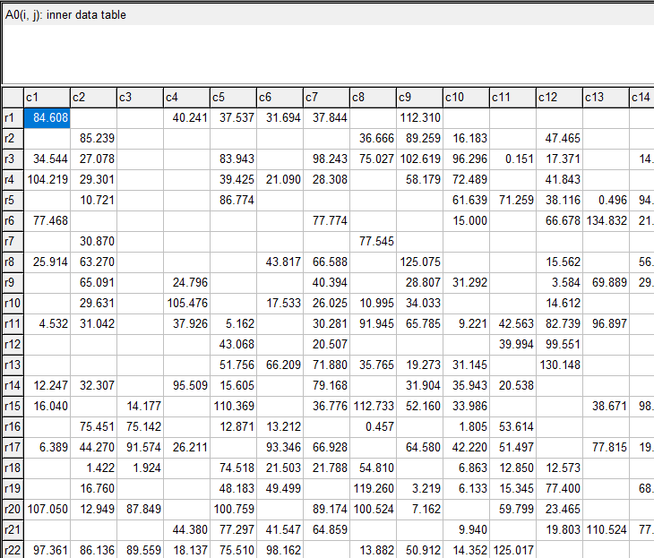
Partial view of the generated matrix \(\color{darkblue}A^0\).

This is not a small problem, with about half a million (non-linear) variables. But this is still way smaller than the problems we may see in practice, especially when we regionalize.

The RAS algorithm


The RAS algorithm for bi-proportional fitting [1] is extremely popular. It is very simple, fast, and converges often in less than 10 iterations. The structure is as follows:

RAS Algorithm
loop

  # row scaling
  \(\rho_i := \displaystyle\frac{r_i}{\sum_j A_{i,j}}\)
  \(A_{i,j} := \rho_i\cdot A_{i,j}\)

  # column scaling
  \(\sigma_j := \displaystyle\frac{c_j}{\sum_i A_{i,j}}\)
  \(A_{i,j} := \sigma_j\cdot A_{i,j}\)

until stopping criterion met


We can stop when an iteration limit is reached or when the quantities \(\rho_i\) and \(\sigma_j\) are sufficiently close to 1.0. In the GAMS code below, we stop either on iterations or on a converge measure.

Below I show the convergence speed by printing the maximum deviation from 1.0 for \(\rho_i\) and \(\sigma_j\). Or in different words: \[\left\|{{\rho-1}\atop{\sigma-1}}\right\|_{\infty}\] 


----     94 PARAMETER trace  RAS convergence

||rho-1|| ||sigm-1|| ||both||

iter1 0.044998550.055590310.05559031
iter2 0.002330510.000123700.00233051
iter3 0.000009580.000000590.00000958
iter4 0.000000043.587900E-90.00000004


---- 95 RAS converged.
PARAMETER niter = 4.000 iteration number


This demonstrates excellent performance. Actually, it is quite astonishing.

Entropy Maximization

The following Entropy based optimization model will give the same solutions as the RAS algorithm above.

The original entropy maximization problem has an objective of the form: \[\max\>H=-\sum_{i,j} b_{i,j} \ln b_{i,j}\] For our RAS emulation, we use a so-called cross entropy form: \[\min\>\sum_{i,j} b_{i,j} \ln \frac{b_{i,j}}{a_{i,j}}\] Our model becomes:


Cross-Entropy Optimization Problem
\[\begin{align}\min&\sum_{i,j|A^0_{i,j}\gt 0}\color{darkred}A_{i,j} \cdot \ln \frac{\color{darkred}A_{i,j}}{\color{darkblue}A^0_{i,j}}\\ & \sum_i \color{darkred}A_{i,j} = \color{darkblue}c_j && \forall j\\ & \sum_j \color{darkred}A_{i,j} = \color{darkblue}r_i && \forall i \\&\color{darkred}A_{i,j}=0 &&\forall i,j|\color{darkblue}A^0_{i,j}=0\\ &\color{darkred}A_{i,j}\ge 0 \end{align} \]

 
To protect the logarithm, I added a small lower bound on \(\color{darkred}A\): \(\color{darkred}A_{i,j} \ge \text{1e-5}\). 

Here are some results:

----    222 PARAMETER report  timings of different solvers

obj iter time

RAS alg -7720.0834.0000.909
CONOPT -7720.083124.000618.656
IPOPT -7720.08315.000171.602
IPOPTH -7720.08315.00025.644
KNITRO -7720.08310.00065.062
MOSEK -7720.05113.00011.125

Notes:
  • The objective in RAS was just an evaluation of the objective function after RAS was finished.
  • In the GAMS model we skip all zero entries. We exploit sparsity.
  • CONOPT is an active set algorithm and is not really very well suited for this kind of models with many super-basic variables. (Super-basic variables are non-linear variables between their bounds).
  • IPOPTH is the same as IPOPT but with a different linear algebra library (Harwell's MA28 instead of MUMPS). That has quite some impact on solution times.
  • MOSEK is the fastest solver, but I needed to add an option: MSK_DPAR_INTPNT_CO_TOL_REL_GAP = 1.0e-5. This may need a bit more fine-tuning. Without this option MOSEK would terminate with a message about lack of progress. I assume it gets a little bit in numerical problems.
  • MOSEK is not a general-purpose NLP solver. We had to use an exponential cone equation. That is a bit more work, and the resulting model is not as natural as the other ones.
  • The difference between the CONOPT solution and RAS solution for \(\color{darkred}A\) is small: 
    ----    148 PARAMETER adiff                =  1.253979E-7  max difference between solutions


Entropy Models [2]


References


  1. Iterative Proportional Fitting, https://en.wikipedia.org/wiki/Iterative_proportional_fitting
  2. Amos Golan. George Judge and Douglas Miller, Maximum Entropy Econometrics, Robust Estimation with Limited Data, Wiley, 1996
  3. McDougall, Robert A., "Entropy Theory and RAS are Friends" (1999). GTAP Working Papers. Paper 6.

Appendix: GAMS Model


$ontext

  
Matrix Balancing:
  
RAS vs Entropy Optimization

$offtext


*---------------------------------------------------------------
* size of the matrix
*---------------------------------------------------------------

set
   i
'rows'/r1*r1000/
   j
'columns'/c1*c1000/
;

*---------------------------------------------------------------
* random sparse data
*---------------------------------------------------------------

Set P(i,j) 'sparsity pattern';
P(i,j) = uniform(0,1)<0.5;

Parameter A0(i,j) 'inner data table';
A0(p) = uniform(0,100);

Parameter
    r(i)
'known row sums'
    c(j)
'known column sums'
;

r(i) =
sum(p(i,j), A0(p));
c(j) =
sum(p(i,j), A0(p));

*
* perturb A0
*
A0(p) = uniform(0.5,1.5)*A0(p);

*---------------------------------------------------------------
* RAS
*---------------------------------------------------------------

set iter 'max RAS iterations'/iter1*iter50/;
Scalars
   tol   
'tolerance'/1e-6/
   niter 
'iteration number'
   diff1 
'max(|rho-1|)'
   diff2 
'max(|sigma-1|)'
   diff  
'max(diff1,diff2)'
   t     
'time'
;

parameters
   A(i,j)
'updated matrix using RAS method'
   rho(i)
'row scaling'
   sigma(j)
'column scaling'
   trace(iter,*)
'RAS convergence'
;

t = timeElapsed;

A(i,j) = A0(i,j);

loop(iter,

    niter =
ord(iter);

*
* step 1 row scaling
*
   rho(i) = r(i)/
sum(j,A(i,j));
   A(i,j) = rho(i)*A(i,j);

*
* step 2 column scaling
*
   sigma(j) = c(j)/
sum(i,A(i,j));
   A(i,j) =  A(i,j)*sigma(j);

*
* converged?
*
   diff1 =
smax(i,abs(rho(i)-1));
   diff2 =
smax(j,abs(sigma(j)-1));
   diff = max(diff1,diff2);
   trace(iter,
'||rho-1||') = diff1;
   trace(iter,
'||sigm-1||') = diff2;
   trace(iter,
'||both||') = diff;

   
break$(diff < tol);

);


option trace:8; display trace;
display$(diff < tol) "RAS converged.",niter;
abort$(niter=card(iter)) "RAS did not converge";

t = timeElapsed-t;

parameter report 'timings of different solvers';
report(
'RAS alg','obj') = sum(p,A(p)*log(A(p)/A0(p)));
report(
'RAS alg','iter') = niter;
report(
'RAS alg','time') = t;

display report;

*---------------------------------------------------------------
* Entropy Model
*---------------------------------------------------------------

variable z 'objective';
positivevariable A2(i,j) 'updated table';

* initial point
A2.l(p) = A0(p);
* protect log
A2.lo(p) = 1e-5;

equations
   objective 
'cross-entropy objective'
   rowsum(i) 
'row totals'
   colsum(j) 
'column totals'
   ;

objective.. z =e=
sum(p,A2(p)*log(A2(p)/A0(p)));
rowsum(i)..
sum(P(i,j), A2(p)) =e= r(i);
colsum(j)..
sum(P(i,j), A2(p)) =e= c(j);

model m1 /all/;
option threads=0, nlp=conopt;

solve m1 minimizing z using nlp;

*---------------------------------------------------------------
* Compare results
* ||A2-A||
*---------------------------------------------------------------

scalar adiff 'max difference between solutions';
adiff =
smax((i,j),abs(A2.l(i,j)-A(i,j)));
display adiff;

*---------------------------------------------------------------
* Try different solvers
*---------------------------------------------------------------

report(
'CONOPT','obj') = z.l;
report(
'CONOPT','iter') = m1.iterusd;
report(
'CONOPT','time') = m1.resusd;

A2.l(p) = 0;

option nlp=ipopt;
solve m1 minimizing z using nlp;

report(
'IPOPT','obj') = z.l;
report(
'IPOPT','iter') = m1.iterusd;
report(
'IPOPT','time') = m1.resusd;

A2.l(p) = 0;

option nlp=ipopth;
solve m1 minimizing z using nlp;

report(
'IPOPTH','obj') = z.l;
report(
'IPOPTH','iter') = m1.iterusd;
report(
'IPOPTH','time') = m1.resusd;

A2.l(p) = 0;

option nlp=knitro;
solve m1 minimizing z using nlp;

report(
'KNITRO','obj') = z.l;
report(
'KNITRO','iter') = m1.iterusd;
report(
'KNITRO','time') = m1.resusd;

display report;

*---------------------------------------------------------------
* for mosek we use the exponential cone
*---------------------------------------------------------------

positivevariable x1(i,j);
variable x3(i,j);
a2.l(p) = 1;

equations
   expcone(i,j)
'exponential cone'
   obj2        
'updated objective'
   defx1       
'x1 = a0'
;


obj2.. z =e= -
sum(p,x3(p));

expcone(p).. x1(p) =g= a2(p)*exp(x3(p)/a2(p));

defx1(p).. x1(p) =e= a0(p);


$onecho > mosek.opt
MSK_DPAR_INTPNT_CO_TOL_REL_GAP = 1.0e-5
$offecho

model m2 /obj2,expcone,rowsum,colsum,defx1/;
option nlp=mosek;
m2.optfile=1;
solve m2 minimizing z using nlp;

report(
'MOSEK','obj') = z.l;
report(
'MOSEK','iter') = m2.iterusd;
report(
'MOSEK','time') = m2.resusd;

display report;


Viewing all articles
Browse latest Browse all 809

Trending Articles